Starting to use Python (and Pandas)¶

Setup plotting¶

To plot data in JupyterLab in a simple fashion use the following code.

%matplotlib inline

This will display plots directly in the notebook. Note, that there are more advanced displaying options for JupyterLab. The allow for example to zoom in.

Load requiered packages¶

Packages offer a wide range of funtionalities, e.g. plotting, calculations, accessing websites with programms. They are mostly listed at pypi.org and can be installed either in a terminal or with the Anaconda distribution.

Terminal:

pip install packageName

Anaconda:

Have a look at the Cheat Sheet (PDF)

For this tutorial, we will need Pandas(Statistics package), Matplotlib(Plotting package) and Numpy(package for numerical work).

Import package¶

After loading the packages, you can access their functionality with the TAB key. If you import the packages like below, the Pandas package e.g. will be available as pd. If you add a DOT pd.and press the TAB key, you will see a list of possible functions.

import matplotlib.pyplot as plt
import pandas as pd
import numpy as np

Test the package access. Uncomment and run the cell. You should see a list of methods.

#pd.

Create a time series¶

Using the Numpy package, we can create a random time series of 1000 entries.

ts = pd.Series(
  np.random.randn(1000),
  index=pd.date_range('1/1/2020',
  periods=1000)
  )

Create a dataset¶

We then create a dataset of random numbers with the time series as an index. Possible columns in the dataset are simply A,B,C and D.

df = pd.DataFrame(
  np.random.randn(1000, 4),
  index=ts.index,
  columns=['A', 'B', 'C', 'D']
  )

df.head(2)

	A	B	C	D
2020-01-01	1.333624	-0.707484	-0.789363	0.152281
2020-01-02	-1.912371	2.753899	-1.315583	0.065484

Calculate cumulative sum¶

We can calculate the cumulative sum of all columns by running

df = df.cumsum()

Have a look at the beginning of the dataset by simply writing df.head(5) and press enter.

df.head(4)

	A	B	C	D
2020-01-01	1.333624	-0.707484	-0.789363	0.152281
2020-01-02	-0.578747	2.046415	-2.104946	0.217766
2020-01-03	-0.173813	1.611432	-2.508927	0.953219
2020-01-04	0.883644	2.065965	-3.386507	1.226043

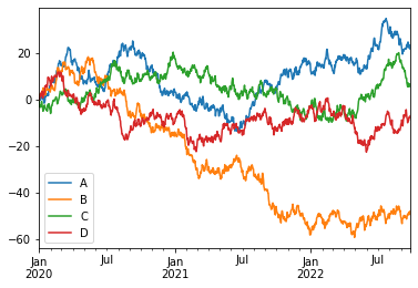
Plot the dataset¶

Since the data is numerical and we have times as index, we can easily create a plot of the dataset by using the .plot() method.

df.plot()

<AxesSubplot:>

This is just to give you a small hint on what can be done with Jupyter Notebooks and Phython. In the course of the book, we will introduce many different useful programms and routines to work with text.

Books as knowledge reservoirs